Enhanced MD sampling
Umbrella Sampling (US)
Background
Umbrella sampling (US; Torrie and Valleau, 1977), like Replica Exchane MD (REMD), helps us to sample conformations that would otherwise be underrepresented. While REMD lets the protein freely explore all space, USMD needs some prior knowledge of the system, a collective variable or order parameter along which we want to steer the simulation. For example, this could be (1) an opening/closing motion of a channel, (2) a rotation of one domain against another, or (3) the distance to a membrane into which we insert the protein. Here, the protein will be restrained in discrete conformations along the collective variable by using harmonic potentials. Thus, we make sure that even high-energy states do not "fall" into the next local minimum. These conformations can be simulated individually, in contrast to REMD, where all replicas must be simulated simultaneously.
Instructions
We will look at the side chains of two charged amino acids, lysine and aspartate, which we expect to behave according to Figure 1 in the paper Debiec et al. In order to eliminate the influence of the backbone, caps were not sufficient, thus the backbone had to be removed and the force field is modified. The modified forcefield can be added to your Gromacs library, but it is sufficient to just copy it into each folder you work with.
1. Preparations
Download the folder us.zip, unzip it and you should have the folders for setup, equilibration, pull, md, usmd and analysis, already with all neccessary files.
2. Generation of the topology files
cd setup
 name="K_D"

	echo 3 | gmx pdb2gmx -f ${name}.pdb -o $name.gro -p $name.top -i ${name}_posre.itp -ter -ff CHARMM27_mod
3. Setup of the system: Box definition and solvation
Since we need a longer distance between our "pull groups" across the periodic boundary conditions than within the box, it is required to choose a large enough box.
 echo 1 | gmx editconf -f $name.gro -o ${name}_box.gro -box 5 3.2 3.2 -princ

	gmx solvate -cp ${name}_box.gro -cs spc216.gro -o ${name}_solvated.gro -p $name.top
Charges are equal and opposite, thus, no neutralization is needed.
4. Energy minimization of the system
 gmx grompp -f em.mdp -po em.out.mdp -c ${name}_solvated.gro -p ${name}.top -o em.tpr

	gmx mdrun -deffnm em
The energy minimization should be instantly finished as the system is very small.
5. Equilibration of the system
Run the equilibration: grompp via console, then the mrun via eq.job (you will have to edit it to your account's path!). This should be finished in a few minutes:
 cd ../eq

	gmx grompp -f eq.mdp -po eq.out.mdp -c ../setup/em.gro -r ../setup/em.gro -t ../setup/em.trr -p ../setup/K_D.top -o eq.tpr

	qsub eq.job
6. Pull MD simulation to generate the different conformations
Copy the resulting files into your pull directory. For the equilibration, all heavy atoms were restrained, but for the production run, we want to restrain one of the two amino acids in place while the other one is pulled away. Gromacs already has the neccessary groups, all we need to do is choose the Lysine for restraining:
echo 2 | gmx genrestr -f eq.gro
Note that the option -DPOSRE_K in the pull.mdp tells Gromacs that we are using restraints. We also need to tell Gromacs in the topology file where exactly these restraints are defined, we do this by adding three lines with vim K_D.top:
	; Include chain topologies
	#include "K_D_Other_chain\_A.itp"
	#ifdef POSRE_K
	#include "posre.itp"
	#endif
	#include "K_D_Other_chain_B.itp"
Next, we will make an index group to define our collective variable as a distance between two atoms:
 gmx make_ndx -f eq.gro -o index.ndx

	> splitat 2

	> splitat 3

    > q
If we look in the pull.mdp, the following options were defined for the pull code:
	pull                = yes
	pull_ncoords        = 1
	pull_ngroups        = 2
	pull_coord1_type    = umbrella
	pull_group1-name    = LYB_NZ_14
	pull_group2-name    = ASB_CG_22
	pull_coord1_groups  = 1 2
	pull_coord1_k       = 1500
	pull_coord1_start = yes
	pull_coord1_geometry = direction
	pull_coord1_vec = 1 0 0
	;Alternative}
	;pull_coord1_geometry = distance
	;pull_coord1_dim = Y Y Y
This block tells Gromacs that, while we let all other forces work as usual, we want to also pull along the vector (1 0 0), with a strength of 1500 kJ/(mol nm2). The groups used for pulling were previously defined in our
index.ndx. We use 1 coordinate for pulling, which needs 2 index groups to be defined. Alternatively, but commented out using a semicolon, we could pull along the vector connecting our two groups, and allow movement in all 3 spatial directions. We prepare the system in order to run the 1 ns pull simulation like this (edit pull.job to your paths!):
 gmx grompp -f pull.mdp -c eq.gro -p K_D.top -t eq.trr -o pull.tpr -r eq.gro -n index.ndx

	qsub pull.job
This takes a little time (around 20 minutes) so this should be run on a cluster or a good computer.
7. Performing an unrestrained MD
To determine the spring constant for our harmonic potentials, it is neccessary to run a normal 2 ns MD simulation. The trajectories for this are provided during the course, unless you want to spend an additional 45 minutes waiting for the simulation. Bonus question: Which parts of the pull.mdp file would you have to change to turn it back into a normal MD?
To analyse our unrestrained MD, I used gmx distance :
gmx distance -s md.tpr -f md.xtc -n index.ndx -select 'com of group "LYB" plus com of group "ASB"' -oall dist.xvg
The console output looked like this:
	Reading frame     600 time  600.000
	Analyzed 629 frames, last time 628.000
	com of group "ASB" plus com of group "LYB":
	   Number of samples:  629
	   Average distance:   1.25566  nm
	   Standard deviation: 0.30779  nm
From which we determine the spring constant κ:
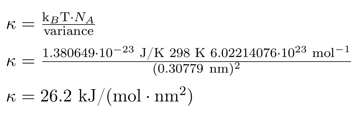
However, experience has taught us that this spring constant is not high enough, which is why you will find a different value in the
us.mdp file later.
Looking at the result of the pulling simulation is possible (on your local machine!) without a gmx trjconv because the position restraints keep our amino acids from drifting:
vmd eq.gro pull.xtc (or vmd eq.gro md.xtc)
Use Mouse > Label > Bonds , then click on the NZ and OD atoms. Go to Graphics > Labels > Bonds, highlight your new distance, go to Graph, and click Graph. In this way, we can see in VMD without actually using gmx distance and xmgrace, how the distances between NZ and OD atoms fluctuate in the simulation. You can also keep in mind that the restraints were defined between NZ and CG, because there are two OD atoms, so this will change the resulting distances slightly.
We will now use the shell script (back on the cluster!) get_distances.sh via gmx distance, which will separate the trajectory into ALL frames, and write out the distance for each frame to the file summary_distances.dat.
To get a graphical output of summary_distances.dat, we need to switch to the local machine, and type:
python myplot.py
However, this is the same as the VMD graph, so we can skip it.
see dist.png
8. Performing the USMD
Now, we are using the pull simulation data, binning our newly acquired conf*.gro files into the umbrella windows. Change the path variables via vim setup.py and then then run
python setup.py.
The output of the script tells us which frames will be used for which window, for example:
	0.1 1 conf4140.gro
	0.2 2 conf122.gro
	0.3 3 conf0.gro
	0.4 4 conf84.gro
	0.5 5 conf1366.gro
	0.6 6 conf1370.gro
	0.7 7 conf1395.gro
	0.8 8 conf1550.gro
	0.9 9 conf1562.gro
For the actual USMD, we will need to run 9 independent 1 ns simulations but we automate this in a job file. First, we need to fill the templates folder:
cp eq/*.itp templates/
cp eq/K_D.top templates/
cp eq/index.ndx templates/
Again, change the paths in the job files:
vim us.job (and vim analysis.job)
and then submit the job (it will take about 1h total):
qsub us.job
If we take another look at the us.mdp, no force to pull is used, while we are still using the pull_coord1_type = umbrella, as before. Instead, we hold each window in place. Once that is finished, we can run the analysis job:
qsub analysis.job
And visualize the results on your local machine using:
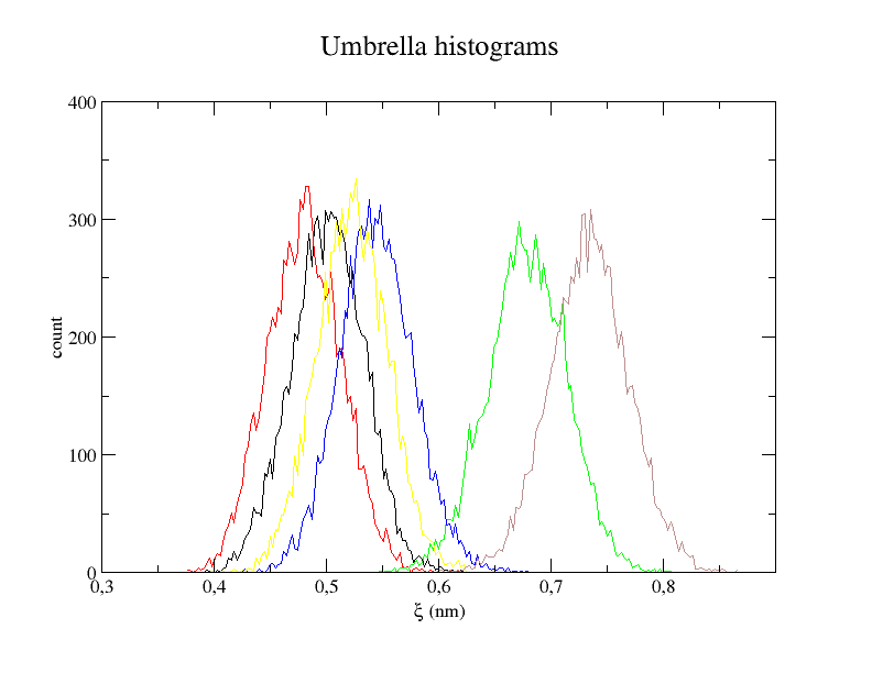
xmgrace -nxy histo.xvg
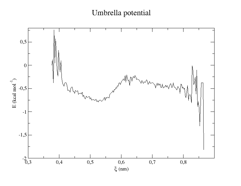
xmgrace profile.xvg
The histogram shows us whether the restraints worked and if the overlap between windows is big enough. The energy profile shows the final result that is an approximation of the potential of mean force between Lysine and Aspartate.