Setup

This section will explain what is needed to set up an MD simulation with Gromacs, starting with peptide coordinates in a PDB file.

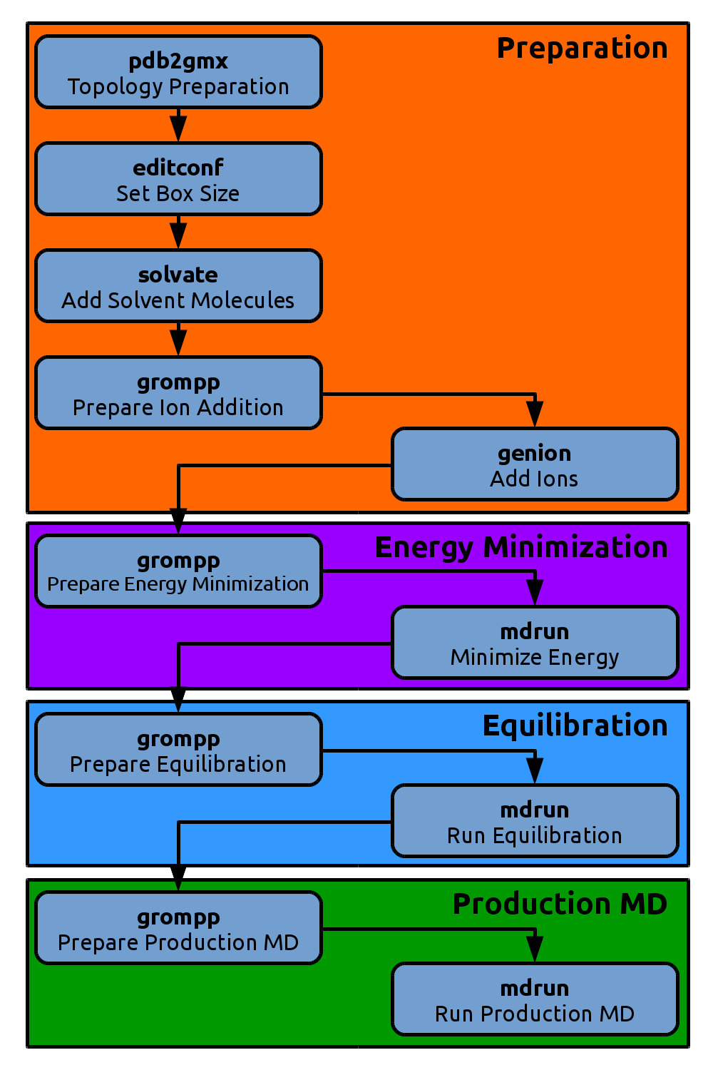
The figures throughout this tutorial give an overview of the current position in the molecular dynamics workflow. They will expand by clicking on them.

Introduction

It takes two ingredients for Gromacs to understand a molecular system: atom coordinates and topology information. The topology file (typically ending in *.top) contains information on how many molecules of which kind a system contains, of what kind their interactions are and the parameters that are used to compute the energy and forces. Gromacs can generate topologies for you. To define a topology, a force field needs to be specified. A force field is a collection of well balanced parameters for the energy and force computation.

Several different families of force fields exist, differing in the way their parameters were derived. Within each familiy, often multiple versions exist, each of which includes corrections to the force field parameters, hopefully making the force field more accurate (within its domain of applicability). But newer versions do not necessarily perform better than their predecessors in all situations. Which force field is good for your purpose depends strongly on your system. For protein systems, the Amber and Charmm force fields are very often a good bet. If you are interested, you can have a look at this historical overview of force field evolution and a review of modern force fields. Protein force fields only contain parameters for standard amino acids, ions and sometimes for nucleic acids and some sugars. If your system contains ligands or unnatural amino acids you will need to find out how to parameterize molecules in accordance your specific choice of force field. In addition to the force field, a water model is also needed. Water is a tough molecule to simulate in classical MD simulations. This is due to the electronic structure of water that gives rise to complex interactions. Several different water models exist. A good overview of water models can be found on the web. It is usually a good idea to stick to a water model that is recommended for your choice of force field or a compatible one.

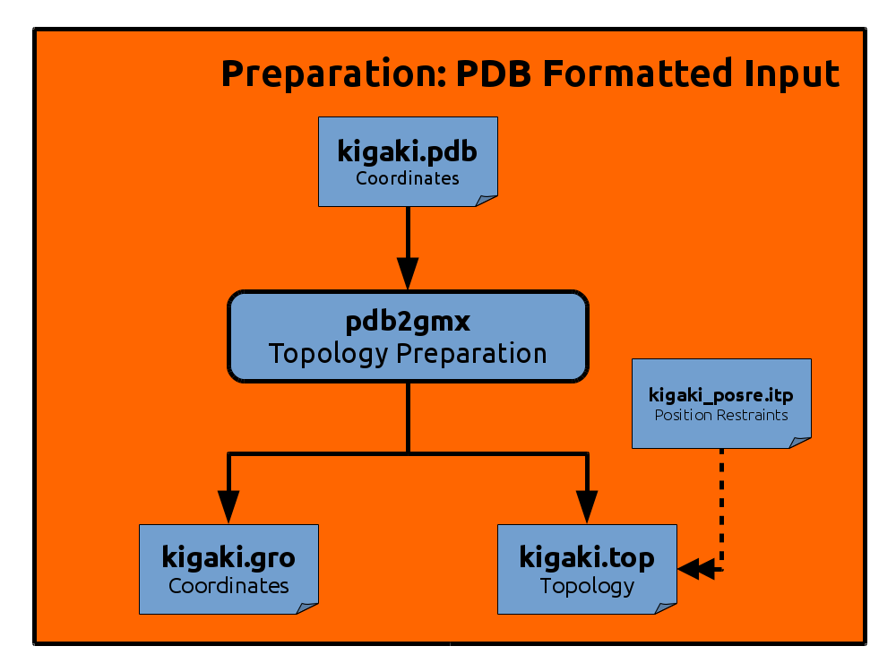
PDB Formatted Input

Download the file kigaki.pdb from the Files section of this tutorial. Open the file with VMD to have a look at the peptide. Now generate a topology with the command below. Choose Amber99sb-ildn as a force field together with the TIP3P water model. While the TIP4P-EW water model performs better in combination with the Amber force fields, it consists of four instead of three particles. To limit the simulation size we will use the TIP3P water model here.

gmx pdb2gmx -f kigaki.pdb -o kigaki.gro -p kigaki.top -i kigaki_posre.itp -ignh

All Gromacs commands work similar. The main program is called gmx and starts every command. It will help you to remember that gmx help commands shows you a list of all available commands with a short description for each of them, while gmx help <command> gives a more detailed description of the tool whose name you substituded for <command>. (Gromacs versions before 5.0 consisted of many programs that have now been merged into gmx. For compatibility reasons it is therefore still possible to omit gmx and directly start with e.g. pdb2gmx, but this not guaranteed to work in the future). The command generated three files. kigaki.gro contains residue and atom names and the coordinates of all atoms. It could in addition contain velocities for the atoms, but at this point we haven’t generated any yet. The second file is the topology file (kigaki.top). Have a look at its contents using the less command. After some comments, this file first includes the parameters of the force field in use:

; Include forcefield parameters #include "amber99sb-ildn.ff/forcefield.itp"

An include directive (#include) instructs Gromacs to substitute the contents of the specified file at that particular position in the topology file. The forcefield.itp file contains the force field parameters of the Amber99sb-ildn force field, which is contained in the Gromacs installation folder. The next section defines molecule types to make them known to Gromacs.

[ moleculetype ] ; Name nrexcl Protein 3

Right now we only have a single protein in our system. If there were more, chain identifiers would be added to the molecule names. The atom section that follows lists all atoms of all residues with some properties like mass and charge. Then some sections follow that specify the bonds, angles, dihedrals and pair (also known as VdW) interactions.
The third file we have generated is kigaki_posre.itp. It contains position restraints for all heavy atoms of the protein, i.e. harmonic potentials that couple the atoms to reference positions. This will be necessary during preparatory steps for the MD simulation to let the water equilibrate around the protein without the protein itself moving significantly, so it cannot get deformed by unequilibrated water molecules. After that, topologies for the water molecules and ions are included as well.
Finally the system is given a name and the number of each molecular species in the system is listed:

[ system ] ; Name Protein in water [ molecules ] ; Compound #mols Protein 1

The latter table will be updated when we add water and ions. The rest of the topology file usually remains constant beyond this point. Consult the Gromacs manual for more information on the layout of topology files. Note that different pH conditions can only be taken into account in a static fashion, that is explicit protonation states need to be specified during this initial setup and remain constant during the simulation. The protonation states of most residues will be set corresponding to neutral pH, while the protonation states of histidines are chosen by pdb2gmx to optimize hydrogen bonding networks.
We have now generated a topological description of our peptide.

Setting the Simulation Box

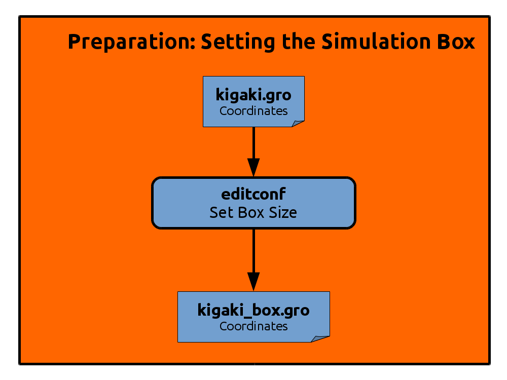
The next step is to create a box around our peptide that we can later fill with solvent. Gromacs can generate boxes of various shapes: triclinical cells, cubes, dodecahedra and octahedra. The triclinical cell has box vectors at right angles, but with different length, while the cubical box has in addition box vectors of equal length. The solute will be centerd in the simulation box with a minimum distance to any wall of 10 Ångstrom (1.0 nm). As the speed of the simulation decreases approximately linearly with the number of particles, we want the box to be as small as possible, but at the same time keep the solute away from its periodic images at all times. The triclinical cell does not work well, as its rectangular shape is problematic for non-globular proteins that might rotate, unless the center of mass rotation is taken care of. We will choose a dodecahedral cell, as it is close in shape to a sphere and minimizes the volume needed to keep the minimum solute to wall distance:

gmx editconf -f kigaki.gro -o kigaki_box.gro -bt dodecahedron -d 1.0

This updated the information about the box that contains our system in the final line of the *.gro file. (You can navigate to the end of a text file in the less program with the G key. g brings you back to the top) The numbers in this final line correspond to the box vector components (in nm) in the order: v1(x) v2(y) v3(z) v1(y) v1(z) v2(x) v2(z) v3(x) v3(y). The latter 6 numbers may be omitted for rectangular boxes and Gromacs only supports boxes with v1(y)=v1(z)=v2(z)=0. Generate some of the other box shapes too and have a look at them with VMD by loading the corresponding *.gro file and typing pbc box in the VMD console. The dodecahedral and octahedral boxes appear not as you might have expected. The reason is that the boxes are always represented in a general, brick shaped unit cell representation for efficiency. Consult the section on periodic boundary conditions in the Gromacs manual to get an idea of how the different representations are transformed into each other.

Learn more about the different box types (popup) offered by Gromacs.

Solvation

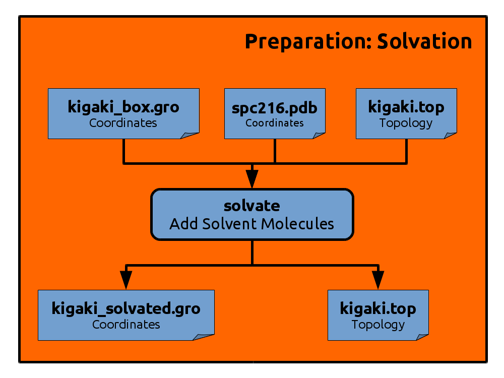
Now the box can be filled with solvent molecules. We have selected the TIP3P water model before, so we need to provide the coordinates of a three-particle water model. As there are no TIP3P coordinates in the Amber force field directories, we will use the coordinates from spc216.gro. This file will be found automatically by Gromacs, without specifying a detailed path. Note that we are still using the correct parameters of the TIP3P water model and only borrowing the coordinates from 216 water molecules, which were produced with the SPC water model.

gmx solvate -cp kigaki_box.gro -cs spc216.gro -o kigaki_solvated.gro -p kigaki.top

Have a look again at the output file in VMD. The solvent box looks brick-shaped for the reason given in the section on box generation. We will later show how to transform the box into its proper octahedral/dodecahedral representation.

Adding Ions

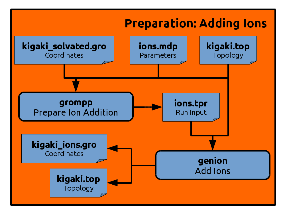
It is also possible to add some ions in order to mimic simulation conditions with specified salt concentrations. However, ions are only approximated as charged point particles and do not possess more detailed electronic structure, which might be relevant for ion binding sites and transition metals ligated to proteins. Though for NaCl the simple point charge description is usually sufficient. We add enough ions to neutralize the system and add an additional concentration of 100 mM NaCl.
For doing so, we need an *.mdp file that contains molecular dynamics parameters. In general, an *.mdp file contains information on the algorithms and options to use during a simulation with Gromacs. It is parsed by the Gromacs preprocessor (grompp) and combined with initial coordinates and velocities into a *.tpr file. *.tpr files contain the complete information that is needed for an energy minimization or any kind of MD simulation with gromacs and is the only required input file for Gromacs' computing engine mdrun.
So why do we need an *.mdp file at this step, as we only want to add ions to our system? Gromacs tries to insert the ions at optimal positions that minimize the energy of the system. Therefore it needs to know which algorithms and parameters to use to compute the energy.

Have a look at the file ions.mdp (popup).

Parse the contents of ions.mdp:

gmx grompp -f ions.mdp -po ions.out.mdp -c kigaki_solvated.gro -p kigaki.top -o ions.tpr -maxwarn 1

As a net charge of the system different from zero could lead to artefacts in combination with the Ewald method, a warning is issued if this should be the case and no files are produced by grompp. However, since the system will be neutralized at the next step, we can ignore this warning which is done with the flag -maxwarn 1. The resulting *.tpr file will be fed into a tool that acually generates the ions:

gmx genion -s ions.tpr -o kigaki_ions.gro -p kigaki.top -pname NA -nname CL -neutral -conc 0.1

When Gromacs asks which molecules to replaced with ions, select the SOL group, which contains all atoms of the solvent (water) molecules. The ions will then be substituted for water molecules at positions that minimize the overall electrostatic energy.

Exercises

Have a look at the resulting system in VMD. The ions can be made visible with the selection keyword ions, using a VdW representation.