Enhanced MD sampling
Replica Exchange MD simulations
Background
One possibility to sample the protein landscape more efficiently is given by the replica exchange molecular dynmaics (REMD) technique. Within the REMD protocol, multiple simulations of the same system (replicas) are run simultaneously at different temperatures. Every τ time steps an attempt is made to swap temperatures between two different replicas i and j (or to swap the protein conformations between the replicas - it does not matter what of the two is swapped). The exchanges are accepted with probability min{1, exp(-Δ)}, where
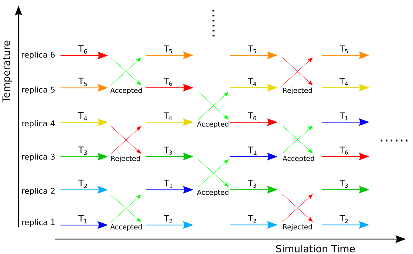
The temperatures for the replicas are typically exponentially spaced between a minimum value Tmin and a maximum value Tmax.
REMD with Gromacs
Detailed information about REMD with Gromacs can be found in the Gromcacs documentation. Here, a step-by-step guide for setting up and running an REMD simulation with implicit solvent using Gromacs is provided.First, the number of the replicas and their temperatures between Tmin and Tmax have to be determined. The number of the replicas depends on the system size and increases as O(f 1/2) for a system with f degrees of freedom (that's why we use an implicit solvent here). The temperatures are usually distributed exponentially (Ti = Tmineki ) since the spacing between replicas can be larger at larger temperatures as the energy distribution of an MD simulation increases with T. The number and temperatures of the replicas have to be chosen such that the expected acceptance probability for exchanges between replicas is about 20%.
In this tutorial an REMD simulation of alanine dipeptide (ala2.pdb) using Amber99sb-ildn as
force field and GBSA as implicit solvent model is prepared. See at the end of this page to find information on how to run
MD simulations with GBSA. The replicas shall be distributed between Tmin = 300 K and Tmax = 500 K.
The .mdp file for the Tmin replica (remd_0.mdp) is provided.
We can use the website REMD temperature generator tool or download the source code published by the authors in PHP language. The following steps based on this website have to be done for running the REMD temperature generator tool:
-
Download the source code as zip file from github site and unzip in a location.
-
We also need to install the php client. Type
phpin the terminal and install it viaapt install. It could be a newer or older version, depending on the linux distribution (here, Ubuntu 2018.04):
sudo apt install php7.2-cli -
Go to the directory remd-temperature-generator-master and type in the terminal:
php -S localhost:8000 -
For the access and starting the application, go to a browser and type in the adress bar:
http://localhost:8000 -
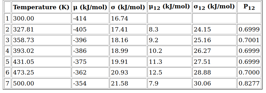
The following pictures shows how to use the REMD temperature generator tool with the corresponding settings (ala2 with 22 atoms; an exchange probability of 0.70; 0 solvent molecules as we use implicit solvent; temperature range between 300 and 500 K). Next, click on submit:

Then, we obtain the following output with the suggestion of 7 replicas and the listed intermediated temperatures with potential energy (μ), the difference between neighbor replicas (index with 12), standard deviation (σ) and the exchange probability (P12):
For each of the replicas we now have to create the input files (.tpr) from the minimized (in the case of explicit solvent:
equilibrated) structure and replica-specific .mdp file. For instance, if we want to run an REMD simulation with 8 replicas with temperatures at 300, 323, 347, 374, 404, 436, 472, and 500 K by using an exchange probability of 0.75, we need eight .mdp files, which we name remd_0.mdp (provided above), ...,
remd_7.mdp. All the parameters contained in these files are the same with the exception of:
     ref_t    = 300.0; for replica 1, i.e. remd_0.mdp
     gen_temp = 300.0; for replica 1, i.e. remd_0.mdp
	     .
	     .
	     .
     ref_t    = 500.0; for replica 8, i.e. remd_7.mdp
     gen_temp = 500.0; for replica 8, i.e. remd_7.mdp
A simple bash loop can be used to generate the eight .tpr files:for i in {0..7}; do gmx grompp -f remd_${i}.mdp -c min.gro -p topol.top -o remd_${i}.tpr; done
Afterwards, the REMD job can be submitted:
mpirun -np 8 gmx_mpi mdrun -s remd_.tpr -multi 8 -replex 1000 -deffnm remd_ -v >& md.out &
Explanations:
    mpirun -np 8 : The number of MPI processes (here 8) that are run in parallel.
    remd_.tpr    : Note that the '_' is not a mistake,
                   it will be automatically extended with the replica number.
    multi        : Instructs Gromacs to perform 8 MD simulations (our replicas).
    replex       : Instructs Gromacs to attempt replica exchanges every 1000 steps.
Note: For REMD an MPI version of Gromacs is required. This can be run across nodes on a computer cluster.
For each replica, a .log file is produced during the REMD simulation. In these files you can find the information about the
replica exchange statistics, such as the exchange probabilities and the number of exchanges per replica pair. For instance:
    Replica exchange statistics
    Repl  4999 attempts, 2500 odd, 2499 even
    Repl  average probabilities:
    Repl     0    1    2    3    4    5    6    7
    Repl      .83  .82  .82  .82  .82  .81  .81
    Repl  number of exchanges:
    Repl     0    1    2    3    4    5    6    7
    Repl     2091 2055 2047 2058 2047 2038 2029
    Repl  average number of exchanges:
    Repl     0    1    2    3    4    5    6    7
    Repl      .84  .82  .82  .82  .82  .82  .81
In this example the exchange probabilities exceed 80%, which is very
high and indicates that similar conformations are sampled in neighbored
replicas.
This is computationally inefficient, thus the number of replicas
should be reduced. If, on the other hand, the exchange probabilities
should
considerably drop below 20%, then the number of replicas is too
small and further replicas need to be added. Here, it is also important
that the exchange probablities are similar across all replica
neighbors. Before submitting the production REMD run it is recommended
to
check with a short test run that the chosen replicas fulfill these
requirements and, if not, to make the necessary adjustments.
Gromacs writes trajectories per temperature (temperature replicas),
which are not continuous with respect to coordinates (as the coordinates
got exchanged during the REMD simulation).
Analysis of REMD simulations
First, we can depict the transitions between the replicas usingdemux.pl:
demux.pl remd_0.log
replica_index.xvg, that can be passed to gmx trjcat, along with the original
trajectory files, in order to produce continuous trajectories, and (2) replica_temp.xvg contains the temperatures for each replica, which
can be opened with xmgrace and we have to zoom in to get a proper overview.Next, we analyze the potential energy for each replica. To this end, you can use a for loop in bash to extract the information and generate the plots:
for i in {0..7}; do echo 10 | gmx energy -f remd_${i}.edr -s remd_${i}.tpr -o Epot_${i}.xvg ; done &> Epot.out & Explanations:
For plotting the data, useecho 10 |: A pipeline is used and your choice (10 for Potential Energy) directly forwarded to Gromacs.&> Epot.out &: All Gromacs output will be written to the file namedEpot.out.
xmgrace Epot_*.xvg .To get nicer curves, you can use the Xmgrace transformation tool
Data > Transformations > running averages.Select all sets and, e.g., 10 or 100 for the length for averaging.
Next, we want to produce a free energy surface (FES) along Φ and Ψ from the REMD data of alanine dipeptide. To do so, follow this protocol:
- Extract the Ramachandran angles Φ and Ψ from each replica
for i in {0..7}; do echo 1 | gmx rama -f remd_${i}.trr -s remd_${i}.tpr -o rama_${i}.xvg ; done &> rama.out & - Produce the files
energies.data,phi.datandpsi.dat, containing the corresponding values for each replica:
 for i in {0..7}; do awk '{if ( $1 !~ /[#@]/) print $2 }' Epot_${i}.xvg > Epot_${i}.dat ; done


    paste Epot_0.dat Epot_1.dat Epot_2.dat Epot_3.dat Epot_4.dat  Epot_5.dat Epot_6.dat Epot_7.dat >  energies.data


    for i in {0..7}; do awk '{if ( $1 !~ /[#@]/) print $1 }' rama_${i}.xvg > phi_${i}.dat ; done


    paste phi_0.dat phi_1.dat phi_2.dat phi_3.dat phi_4.dat phi_5.dat phi_6.dat phi_7.dat > phi.dat


    for i in {0..7}; do awk '{if ( $1 !~ /[#@]/) print $2 }' rama_${i}.xvg > psi_${i}.dat ; done


paste psi_0.dat psi_1.dat psi_2.dat psi_3.dat psi_4.dat psi_5.dat psi_6.dat psi_7.dat > psi.dat - Produce the FES using
wham.
For the production of the FES, you need the wham program and the file histo.para. Important here, thewham programbased on Gfortran 3, so you might install gfortran (sudo apt-get install gfortran) and this library (sudo apt-get install libgfortran3). This is working until Ubuntu 18.04 otherwise the program does not work.Make sure that
whamis an executable file:chmod 744 wham
Adjust the settings inhisto.parato reflect the details of your REMD simulation: number of replicas, replica temperatures, number of data points.
Then execute thewhamprogram:./wham phi.dat psi.dat <temperature>
where<temperature>has to be replaced by the temperature value at which the FES should be generated, e.g., 300 K. Several files are produced, of whichF_R1_R2.datcontains the free energies along Φ and Ψ, which can be plotted usinggnuplot.
Hint: Before generating a new FES at, e.g., another temperature, copyF_R1_R2.datto, e.g.,FES_, otherwise your previous file will be overwritten!.dat
MD with implict solvent
As in the example above, an REMD simulation with implicit solvent is set up, a short description of how to run an MD simulation with GBSA as implicit solvent using Gromacs is provided here. As the latest Gromacs versions do no longer support GBSA, we have to use an older Gromacs version: Gromacs version 5.1.1.
Three steps are required for running an implicit MD simulation with Gromacs:
- Generate the topology file:
gmx pdb2gmx -f ala2.pdb -ter -ignh -interSelect the force field,
Amber99sb-ildn, andNonefor the water model. It will generateconf.groandtopol.topas output. - Energy minimization using min-implicit.mdp:
gmx grompp -f min-implicit.mdp -c conf.gro -p topol.top -o min.tpr
gmx mdrun -deffnm min -v >& min.out &Note: There is no need to set up a box, add ions, or perform position restraint dynamics (equilibration) when using an implicit solvent MD simulation as i) no periodic boundary conditions are employed and ii) there can be no clashes between the protein and water molecules.
- Production run using md-implicit.mdp:
gmx grompp -f md-implicit.mdp -c min.gro -p topol.top -o imd.tpr
gmx mdrun -deffnm imd -v >& imd.out &